From the Sigmoid to the First Neuron#
In the previous lesson, our watering model learned to calculate a score from temperature and humidity.
We had:
temperature
      +
humidity
      ↓
  parameters
      ↓
     score
      ↓
   decision
But something bothered us.
Our model could produce:
-4.93
0.01
3.05
Then we simply asked it:
if score > 0 → water
otherwise    → do not water
That works for making a decision.
But we immediately lose information.
A score of 0.01 and a score of 8 both give the same answer:
water
Yet those two scores clearly do not tell the same story.
So we ended the previous lesson with a question:
How can we transform our score into an output between 0 and 1?
Let’s try.
A function between 0 and 1#
We are looking for a function that can receive any score and bring it back between 0 and 1.
One function is particularly well suited to this job: the sigmoid.
Its formula is:
sigmoid(x) = 1 / (1 + exp(-x))
It may look a little less welcoming than our usual score.
Rather than dissecting it immediately, let’s look at what it does.
During our previous experiment, we calculated a few values:
| Score | Sigmoid |
|---|---|
| -4 | 0.018 |
| -2 | 0.119 |
| -1 | 0.269 |
| 0 | 0.500 |
| 1 | 0.731 |
| 2 | 0.881 |
| 4 | 0.982 |
The first thing we notice is that negative scores give values below 0.5.
Positive scores give values above 0.5.
And exactly in the middle:
sigmoid(0) = 0.5
Let’s go a little further.
For a score of 8, we obtained:
sigmoid(8) = 0.9996646498695336
So we are very close to 1.
Very close.
But still not 1.
Our sigmoid seems decidedly reluctant to make absolute decisions.
In the other direction, it behaves the same way: it gets closer and closer to 0 without reaching it.
A curious S-shaped curve#
The numbers already give us a clue.
The graph makes the behavior much easier to see.
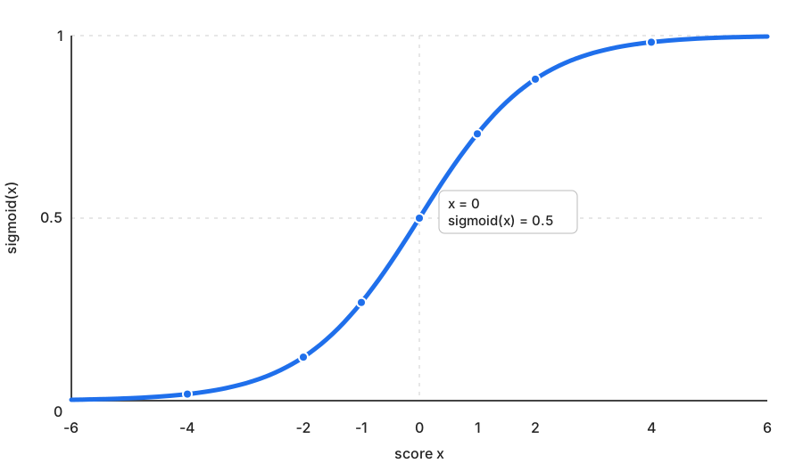
y = 1 / (1 + exp(-x))
We can find our values again on this curve.
On the left, it gradually approaches 0.
In the center:
x = 0
y = 0.5
On the right, it gradually approaches 1.
And most importantly, the curve is much more sensitive around its center.
That is exactly the property we were looking for.
Our score is no longer abruptly turned into 0 or 1.
We keep an intermediate value.
Back to watering#
We already know the parameters learned earlier:
temperature weight = 0.38
humidity weight    = -0.19
bias               = 0.01
Let’s try:
temperature = 28 °C
humidity    = 40 %
Our usual calculation gives:
score = 28 × 0.38
      + 40 × (-0.19)
      + 0.01

score = 3.05
Now pass 3.05 through the sigmoid.
We obtain:
0.9547825265167125
About 0.955.
We are clearly on the side of 1.
Now keep 28 °C, but raise humidity to 80 %.
This time:
output ≈ 0.010
We are almost at the other end.
That fits our watering problem fairly well:
output close to 0 → do not water
output close to 1 → water
But what happens between the two?
Let’s find the boundary#
Keep the temperature at 28 °C.
Then vary humidity.
Around 56 %, we obtained:
28 °C / 55 % → 0.5498
28 °C / 56 % → 0.5025
28 °C / 57 % → 0.4551
Now this is much more interesting.
At 55 %, our output is slightly above 0.5.
At 57 %, it is slightly below.
And at 56 %:
0.5025
Our model is practically sitting on the fence.
Yet at some point we still have to decide which side to fall on.
We can choose a rule:
output >= 0.5 → water
output <  0.5 → do not water
But that decision rule comes after the sigmoid.
The sigmoid itself keeps the nuance.
It lets us distinguish an output of 0.5025 from an output of 0.9548.
So we have solved our first problem.
Our score has become a continuous output between 0 and 1.
But now let’s look at the program we have been building.
What have we built?#
We already had this:
temperature ──× weight ──┐
                         │
humidity ─────× weight ──┼──> score
                         │
bias ────────────────────┘
We have just added:
score ──> sigmoid ──> output
Put the two together:
temperature ──× temperature_weight ──┐
                                       │
humidity ─────× humidity_weight ───────┼──> score ──> sigmoid ──> output
                                       │
bias ──────────────────────────────────┘
Look at what we have.
We have inputs.
Each input has a weight.
We add a bias.
We calculate a score.
Then we pass that score through an activation function.
This is starting to look suspiciously like something.
We have just built our first artificial neuron.
And we did it almost without noticing.
Our neuron in Python#
The corresponding program is actually very short:
import math


temperature_weight = 0.38
humidity_weight = -0.19
bias = 0.01


def sigmoid(x):
    return 1 / (1 + math.exp(-x))


def neuron(temperature, humidity):
    score = (
        temperature * temperature_weight
        + humidity * humidity_weight
        + bias
    )

    return sigmoid(score)
Our neuron() function receives two inputs and returns an output.
We can then apply our decision rule:
output = neuron(28, 40)

if output >= 0.5:
    print("water")
else:
    print("do not water")
So now we know what our first neuron is.
But there is still one small problem.
And it is a rather important one.
We wrote:
temperature_weight = 0.38
humidity_weight = -0.19
bias = 0.01
Where did those values come from?
Who sets the weights?#
We already know part of the answer.
Our neuron has five examples:
| Temperature | Humidity | Target |
|---|---|---|
| 22 | 70 | 0 |
| 24 | 65 | 0 |
| 27 | 42 | 1 |
| 29 | 35 | 1 |
| 25 | 55 | 0 |
For each one, it produces an output.
We also know the target.
So we need to measure how far the two are from each other.
That should sound familiar.
In Lesson 03, we used a loss function.
Let’s use the same idea again:
error = target - output
loss = error²
We do not need to invent a new mechanism.
We have our neuron.
We have a target.
And now we know how to measure its error.
A familiar question returns:
In which direction should we change the parameters to make this loss smaller?
An old tool returns#
Take only the temperature weight.
Its current value is:
0.38
During our experiment, we moved it very slightly around that value:
0.379 → loss ≈ 0.0866
0.380 → loss ≈ 0.0890
0.381 → loss ≈ 0.0916
When we increase the weight slightly, the loss increases.
So we know something about the slope at that point.
And that slope has a name we already know:
the gradient.
We have found the same idea as gradient descent again.
This time, it will help us adjust the parameters of our neuron.
We use the same reasoning for the humidity weight and the bias.
Then we can correct them.
Let’s try.
A first step… slightly too enthusiastic#
Start with:
learning_rate = 0.01
Our loss before the correction is about:
0.089041
After correcting all three parameters:
0.505459
We wanted to go down.
We went up.
And not by a little.
The local direction gave us useful information, but our step was clearly too large.
Let’s try ten times smaller:
learning_rate = 0.001
This time:
0.089041 → 0.060073
That looks much more like a descent.
So we have rediscovered another idea from the previous lessons: knowing the direction is not enough.
We also need a suitable step size.
Let’s continue#
Now that our first step goes in the right direction, repeat it.
After ten small steps, we observed:
start          0.089041
iteration 1    0.060073
iteration 2    0.052935
iteration 3    0.050631
...
iteration 10   0.048669
The loss does not magically disappear.
But it goes down.
The parameters have changed slightly too:
temperature weight ≈  0.3769
humidity weight    ≈ -0.2035
bias               ≈  0.0098
Good.
But after all those calculations, one question is much more interesting than the sixth decimal place of our loss:
What can our neuron do now?
Let’s look at its outputs instead#
After those ten iterations:
| Temperature | Humidity | Target | Output |
|---|---|---|---|
| 22 | 70 | 0 | 0.003 |
| 24 | 65 | 0 | 0.015 |
| 27 | 42 | 1 | 0.838 |
| 29 | 35 | 1 | 0.979 |
| 25 | 55 | 0 | 0.147 |
All five observations are now on the expected side of 0.5.
So the three numerical values we initially placed in our program were not fixed forever.
The neuron can correct them from examples.
What is actually learned is:
the weights
the bias
The loss itself is not learned.
It is a measurement we use to see how the model behaves and to guide the corrections.
One last caution is necessary.
An output of:
0.838
is indeed between 0 and 1.
But we have not demonstrated that it means:
83.8 % probability that we should water
For now, it mainly tells us which side of our chosen boundary the observation lies on, and how far it is from 0.5.
What we have just built#
We started with a very simple problem:
our model produces a score
We wanted to keep more information before making a decision.
We discovered the sigmoid.
Then, almost without looking for it, we ended up with:
inputs
   ↓
weights + bias
   ↓
score
   ↓
sigmoid
   ↓
output
That was our first neuron.
One question remained:
who sets its weights?
And to answer it, we did not need to start over.
We found the tools from the previous lessons again:
output
   ↓
target
   ↓
loss
   ↓
gradient
   ↓
correction of weights and bias
   ↓
new output
So we have not entered a completely different world.
We have simply assembled, one by one, pieces we already knew.
And this time, their combination has a name:
an artificial neuron that learns.
We still have only one.
So a new question appears quite naturally:
What might happen if several neurons worked together?